Project 1

Biden’s Approval Margins

As we saw in class, fivethirtyeight.com has detailed data on all polls that track the president’s approval

# Import approval polls data directly off fivethirtyeight website
approval_polllist <- read_csv('https://projects.fivethirtyeight.com/biden-approval-data/approval_polllist.csv') 

glimpse(approval_polllist)

## Rows: 4,596
## Columns: 22
## $ president           <chr> "Joe Biden", "Joe Biden", "Joe Biden", "Joe Biden"…
## $ subgroup            <chr> "All polls", "All polls", "All polls", "All polls"…
## $ modeldate           <chr> "9/20/2022", "9/20/2022", "9/20/2022", "9/20/2022"…
## $ startdate           <chr> "1/19/2021", "1/19/2021", "1/20/2021", "1/20/2021"…
## $ enddate             <chr> "1/21/2021", "1/21/2021", "1/21/2021", "1/22/2021"…
## $ pollster            <chr> "Morning Consult", "Rasmussen Reports/Pulse Opinio…
## $ grade               <chr> "B", "B", "B", "B", "B+", "B-", "B-", "B+", "B", "…
## $ samplesize          <dbl> 15000, 1500, 1993, 15000, 1516, 1115, 1200, 941, 1…
## $ population          <chr> "a", "lv", "rv", "a", "a", "a", "rv", "rv", "a", "…
## $ weight              <dbl> 0.2594, 0.3382, 0.0930, 0.2333, 1.2454, 1.1014, 0.…
## $ influence           <dbl> 0, 0, 0, 0, 0, 0, 0, 0, 0, 0, 0, 0, 0, 0, 0, 0, 0,…
## $ approve             <dbl> 50.0, 48.0, 56.0, 51.0, 45.0, 55.5, 58.0, 63.0, 52…
## $ disapprove          <dbl> 28.0, 45.0, 31.0, 28.0, 28.0, 31.6, 32.0, 37.0, 29…
## $ adjusted_approve    <dbl> 49.4, 49.1, 55.4, 50.4, 46.0, 54.6, 57.5, 59.4, 51…
## $ adjusted_disapprove <dbl> 30.9, 40.3, 33.9, 30.9, 29.0, 32.4, 32.7, 38.4, 31…
## $ multiversions       <chr> NA, NA, NA, NA, NA, NA, NA, NA, NA, NA, NA, NA, NA…
## $ tracking            <lgl> TRUE, TRUE, NA, TRUE, NA, NA, NA, NA, TRUE, TRUE, …
## $ url                 <chr> "https://morningconsult.com/form/global-leader-app…
## $ poll_id             <dbl> 74272, 74247, 74246, 74273, 74327, 74248, 74270, 7…
## $ question_id         <dbl> 139491, 139395, 139394, 139492, 139570, 139404, 13…
## $ createddate         <chr> "1/28/2021", "1/22/2021", "1/22/2021", "1/28/2021"…
## $ timestamp           <chr> "17:52:31 20 Sep 2022", "17:52:31 20 Sep 2022", "1…

# Use `lubridate` to fix dates, as they are given as characters.

library(lubridate)
approval_polllist <- approval_polllist %>% 
  mutate(enddate = mdy(enddate),
         startdate = mdy(startdate),
         modeldate = mdy(modeldate),
         week = week(enddate))

Create a plot

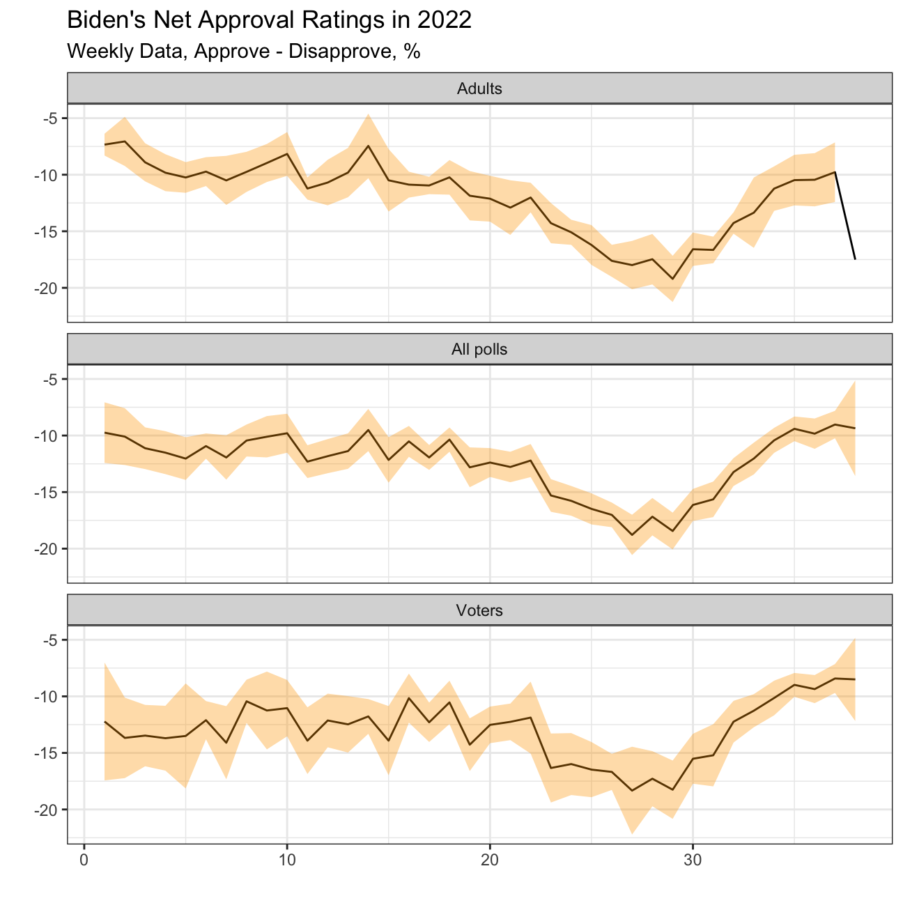
What I would like you to do is to calculate the average net approval rate (approve- disapprove) for each week since he got into office. I want you plot the net approval for each week in 2022, along with its 95% confidence interval. There are various dates given for each poll, please use enddate, i.e., the date the poll ended. Your plot should look something like this:

approval_polllist %>% 
  mutate(year = year(enddate)) %>% 
  filter(year == 2022, week<50) %>%
  mutate(net_approval_rate = (approve-disapprove)) %>% 
  group_by(week, subgroup) %>% 
  summarise(
    mean_net_approve = mean(net_approval_rate),
    sd = sd(net_approval_rate),
    count = n(),
    se = sd/sqrt(count),
    lower95 = mean_net_approve - qt(0.975,count-1)*se,
    upper95 = mean_net_approve + qt(0.975,count-1)*se) %>% 

ggplot(aes(x = week, y=mean_net_approve))+
  geom_line()+
  facet_wrap(~subgroup, nrow=3)+
  geom_ribbon(aes(ymin = lower95, ymax = upper95), alpha=0.35, fill = "orange", 
             linetype = "solid", nrow=3)+
  theme_bw()+
  labs(title = "Biden's Net Approval Ratings in 2022",
    subtitle = "Weekly Data, Approve - Disapprove, %",
    y= "", 
    x = ""
  )